
Large graphs can take a lot of memory. We can use Binary Decision Diagrams to reduce the space complexity. We will first convert the graph into a boolean formula, and then convert that formula into a Binary Decision Diagram (which in itself is a graph). As there are not many “practical” guides for BDDs out there, I thought that I would create this post to clarify how to construct and use BDDs by stepping through an example using Python.
Let’s look at an example graph:
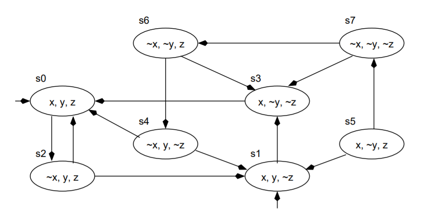
In order to convert this graph to a boolean formula, we first need to represent each variable as a combination of binary variables. Since we have 8 nodes, we will need 3 binary variables to represent all our nodes. Let \(x_1, x_2,\) and \(x_3\) be our binary variables. The nodes can be represented as binary variables as follows:
| Original node | \(x_1\) | \(x_2\) | \(x_3\) |
|---|---|---|---|
| s0 | 0 | 0 | 0 |
| s1 | 0 | 0 | 1 |
| s2 | 0 | 1 | 0 |
| s3 | 0 | 1 | 1 |
| s4 | 1 | 0 | 0 |
| s5 | 1 | 0 | 1 |
| s6 | 1 | 1 | 0 |
| s7 | 1 | 1 | 1 |
The boolean formula to represent \(s5\) is \(x_1 \wedge \neg x_2 \wedge x_3\). Now that we have represented the nodes into boolean formulas, we next move onto how to represent the edges. Two nodes are needed to describe an edge. We will use the boolean variables \(x_1, x_2, x_3\) for the initial node, and \(x_4, x_5, x_6\) for the terminal node (so now we are using 6 boolean variables). Let’s consider the edge \(s6 \rightarrow s4\) which is denoted as \(R_{6,4}\). The boolean formulae for \(s6\) and \(s4\) are \(x_1 \wedge x_2 \wedge \neg x_3\) and \(x_4 \wedge \neg x_5 \wedge \neg x_6\) respectively. The edge is represented as the conjunction of these formulae: \(R_{6,4} = x_1 \wedge x_2 \wedge \neg x_3 \wedge x_4 \wedge \neg x_5 \wedge \neg x_6\).
Since there are 13 edges in this graph, we will have 13 similar formulae. The disjunction of these edge formulae will give us a boolean formula (\(R\)) for the whole graph. Or in other words \(R = R_{0,2} \vee R_{1,3} \vee ... \vee R_{7,6}\). We can represent this boolean formula in a nice compact format using a BDD. Traversing the BDD will show what edges are in a graph. A path terminating in 1 means that the edge is in the original graph. However, if a path terminates in 0, that means that the edge is not in the original graph. The BDD for our graph can be seen below:
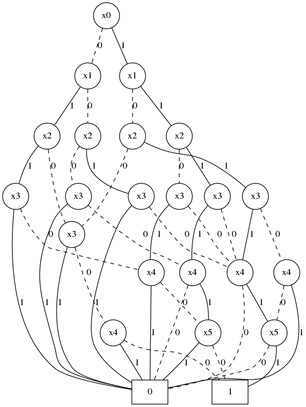
Notice that this is a directed acyclic graph. Now that we have represented the graph as a BDD, we can perform different graph searches and model checking algorithms. I will update this article to include how to perform symbolic model checking.
Implementation in Python
Let’s implement this using the pyeda package in Python. This will also be done in jupyter notebooks to break our implementation into steps, and to help us visualize better what’s going on.
First I will import the packages needed. pyeda will be used to make and work with the BDDs, pandas will be used to store the edges, and graphviz will help us visualize the BDDs:
from pyeda.inter import *
import pydot
import graphviz
import pandas as pd
%load_ext gvmagic
The edges will be stored as strings in a list. I will need to convert all of these edges to a boolean formula. I first convert this list to a pandas dataframe.
R = ['000010','010000','100000','011000','110100','100001','010001','001011','101001','101111','111110','111011','110011']
Rs = []
for s in R:
    Rs.append([int(e) for e in s])

R = pd.DataFrame(Rs)
Each row of the R dataframe now represents an edge. convert_bin_formula(R) converts the R dataframe as a boolean formula.
def convert_row_to_formula(row):
    row_formula = ['~'*abs(row[i]-1) + f'x{i}' for i in range(len(row))]
    return ' & '.join(row_formula)

def convert_bin_formula(R):
    r_formulas = []
    for row in R.iterrows():
        r_formula = convert_row_to_formula(row[1])
        r_formulas.append(r_formula)
    return ' | '.join(r_formulas)

expression = convert_bin_formula(R)
Next, we will represent the boolean formula of the graph as a BDD. The expr and expr2bdd functions from the pyeda module will convert our expression to a boolean formula, and convert our boolean formula to a BDD respectively.
f = expr(expression)
f = expr2bdd(f)
All done! We have converted a graph to a BDD. If you are using Jupyter Notebooks, you can display this BDD using the magic command %dotobj f. You can also output the BDD as a dot file using f.to_dot().